The Autonomous Outbound Worker Part 1

This is the first post in a series on our research into autonomous outbound. With hiddenweights, we built the Rox Outbound Reward Model, a small model that scores cold emails the way SDRs do. It agrees with real SDR edits 80% of the time, where GPT and Claude score below 50%, and it runs faster and cheaper than either.

Rox in collaboration with hiddenweights.

Authors: Gopal Goel, Calvin Yost-Wolff, Marcus Dominguez-Kuhne. Andrew Ilyas, Mina Farid, Hedi Driss, and the team at Hiddenweights.

01: The Outbound Task

Outbound sits at the top of the revenue funnel and is often the first surface that new prospects interact with. A company decides which customers it wants and begins conversations with them from a cold start, with the main goal of booking introductory meetings.

We built an Autonomous Outbound Worker that, given a contact and an outreach reason, writes, sends, follows up, and adapts until a meeting is booked. Improving it requires solving open research problems unique to sales. This series follows the iterations and breakthroughs we achieved along the way.

Our first problem: giving the agent a reliable reward signal for outbound. In collaboration with hiddenweights, we built the Rox Outbound Reward Model, a 3B-scale model trained on pairs of emails before and after an SDR edited them, then tuned on sparse signals like opens and replies. Compared with GPT and Claude used as judges:

1. It agrees with SDRs. On 717 held-out SDR edits, it rates the edited version higher 80% of the time. GPT and Claude score 38% and 45%, below a coin flip.

2. Its scores track replies. The emails it scores in the top 20% get 1.75× the average reply rate. The judges' scores barely move with replies.

3. It's faster and cheaper. About 0.37 seconds and $0.06 per 1,000 emails, against 1.9–2.2 seconds and $0.27–$1.77 for the judges.

Here is what that looks like in practice. For one fictional prospect, we generated 100 drafts and let the model pick (Figure 1). The pick is more direct and ends with a simpler ask. Section 07 shows how the selection works.

Figure 1: One fictional request (Maya Okafor, VP of Sales at Brightwell Freight, after a $38M Series B and six new SDR roles). Left: one of 100 drafts from claude-sonnet-5, chosen at random (reward −5.0, 12th percentile of held-out real sends). Right: the draft the reward model scored highest (reward 7.8, 51st percentile).

02: The Signal Problem

Agents are extraordinarily good at hill-climbing verifiable, dense rewards. Coding is the clearest example: give a model a test suite and an environment to iterate in, and it will likely pass the tests. The pattern holds for most problems where success can be checked automatically.

Outbound has no such check. The obvious candidate is reply rate, but three things make it unusable as a direct training signal:

1. Sparsity. A well-run email sequence gets about a 1–2% reply rate.

2. Delay. If a meeting gets booked after the fourth email in a sequence, twelve days after the first, which email earned it?

3. Confounding. Signal quality, persona fit, contact data accuracy, sender reputation, and time of year all move replies, and the email controls none of them.

A useful reward needs to be dense, available immediately, and strongly correlated with replies. The other measurable proxies fail the same way, and some teach bad habits: optimize for open rate, and the agent learns to write clickbait subject lines.

03: Edits as Training Data

Since the early days of Rox, SDRs have used the product to draft emails and then done one of three things: send as-is, edit and send, or discard. Our key realization is that every one of these actions is a label from a domain expert, produced at the moment of generation, at zero additional cost to collect. An SDR who edits your email is telling you, character by character, what was wrong with it. Nothing else in the outbound data pipeline provides feedback this specific, this fast, or from someone this qualified.

With hiddenweights, we turn these before-and-after pairs into a reward model: a model that reads only the email text and returns a single score for its style. We train it with the Bradley-Terry loss, which pushes the model to score each edited email higher than the draft it replaced:

Equation 1: pipi​ is the model's probability that the edited version of pair ii beats the original; σσ is the sigmoid function. Training minimizes the loss ℓiℓi​ across all pairs.

Edits alone already go a long way: a model trained on nothing else produces scores that track replies (Figure 4).

04: Scaling Beyond Real Edits

Real edits are the best signal in sales, but there are relatively few of them, and they cover a narrow slice of the market. A model trained only on that slice can look accurate on familiar emails and fail on new ones. Synthetic data can widen coverage, but only if it is unfamiliar enough to harden the model while still looking like something an SDR would actually write.

hiddenweights' optimized synthesizer handles this. It probes the reward model for blind spots and generates synthetic edit pairs that target them, each with a weight that sets how much that pair counts during training.

Choosing those weights is the hard part. We hold out a small set of high-quality real edits as a target set, and the goal is to pick weights so the trained model does as well as possible on it. But every weight influences every step of training, so the effect of a single weight on the final model runs through a very long chain of computation (Figure 2).

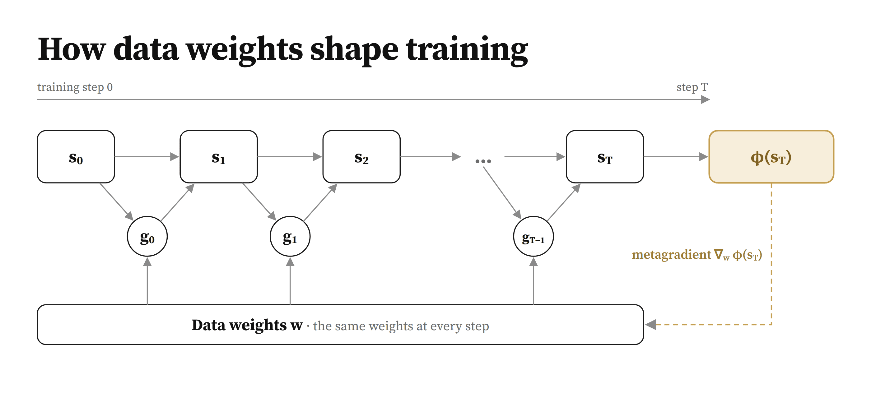
Figure 2: Training unrolled over time. Each gradient step gtgt​ moves the model from state stst​ to st+1st+1​, and every step is shaped by the same data weights ww. The metagradient \( abla_w arphi(s_T)\) traces how the final result depends on those weights, back through every step. Adapted from Ilyas and Engstrom (2025).

The synthesizer solves this with metagradient descent: it differentiates the target-set performance through the entire training run, ∇wφ(sT)∇w​φ(sT​), and uses that gradient to update the weights.

Metagradients work for any objective, which lets us fold in replies and opens even though they are too sparse to train on directly. Our final objective rewards agreeing with held-out SDR edits and scoring opened and replied emails higher:

Equation 2: The final meta-objective. ℓjℓj​ is the Bradley-Terry loss from Equation 1 on target-set pair jj; the engagement term uses that email's open and reply data ejej​, favoring higher scores for emails that got engagement and lower scores for those that didn't.

Edits supply dense expert judgment; opens and replies, however noisy, measure what the market actually responds to. The final model learns from both.

05: What the Model Learned

First, a sanity check. We applied simple edits to 2,000 synthetic cold emails, one at a time, and measured how the score moved. Every edit moved it in the direction an SDR would expect: breaking a dense block into short paragraphs helps; lowercasing everything, a casual "Hey," or a generic company-bragging paragraph hurts.

Figure 3: Mean change in reward when one edit is applied to each of 2,000 synthetic cold emails, with 95% confidence intervals. The right column shows the share of emails whose score moved in the expected direction. One standard deviation of reward on held-out sends is 8.5 points.

The real test is replies. On 33,933 held-out sends (Aug 29 – Sep 24, 510 replies), kept separate from all training data, higher scores meant more replies. That holds even for the model trained on edits alone, and adding engagement makes the link stronger: each standard deviation of reward raises the odds of a reply by 1.77×, up from 1.53×.

Figure 4: Every held-out send at its reward, for the edits-only model (top) and the final model with engagement (bottom). Top: reply rate implied by the score (logistic fit, 95% band) and the observed rate in each tenth of emails. Bottom: emails that got a reply versus those that didn't, with each group's median.

06: Beating Frontier Judges

The most obvious way to score emails is to ask a frontier model. Since the most capable models are too expensive to run on every draft in production, we tested GPT-5.6-luna and Claude Sonnet 4.6, each asked to score emails from 0 to 100.

Start with the task the reward model was trained for: agreeing with SDRs. On 717 held-out edits, we asked each scorer whether the edited version was better than the original. Both versions of our model agree about 80% of the time. GPT-5.6-luna and Claude Sonnet 4.6 come in at 38% and 45%, worse than a coin flip.

Figure 5: The same 717 held-out SDR edits (sent Aug 29 – Sep 23) for every scorer: the share where it scored the edited version higher, the same, or lower than the original. Win rate counts ties as half; 50% (dotted) is a coin flip. Brackets show 95% bootstrap intervals.

The judges' scores also say little about replies. Under both, the emails that got a reply and the ones that didn't have the same median score: 72.

Figure 6: The two LLM judges, shown the same way as Figure 4: GPT-5.6-luna (top) and Claude Sonnet 4.6 (bottom). These are 3,430 SDR-edited emails with 57 replies, a smaller set than Figure 4's, so the intervals are wider.

Put another way: keep only the emails each scorer ranks in its top 20%, and our model's picks get 1.75× the average reply rate. GPT's get 1.33× and Claude's 1.23×, with intervals wide enough to include no lift at all.

Figure 7: Reply rate of each scorer's top-scored emails relative to the average, as fewer emails are kept. The band is the 95% interval for the final model. At the top 20%, the lifts are 1.75× (final model), 1.64× (edits only), 1.33× (GPT) and 1.23× (Claude). Reward models are evaluated on 33,933 held-out sends (510 replies); judges on 3,430 SDR-edited emails (57 replies).

It is also faster and cheaper to run than either judge (Table 1).

Table 1: Mean latency per scoring call and cost per 1,000 emails. The reward model figures come from an older version of the model on its shared production endpoint, with cost estimated from GPU time; judge costs are list prices applied to their token counts.

07: Putting It to Work

Figure 8: Best-of-N generation: the agent drafts N candidate emails, the reward model scores each one, and the top-scoring draft is sent.

An instant score lets the agent compare drafts before anything is sent. The simplest use is best-of-N: write many candidates, score them all, and send the best (Figure 8). Figure 9 shows it on the fictional request from Figure 1: of 100 drafts, the reward model's pick lands far above the typical draft.

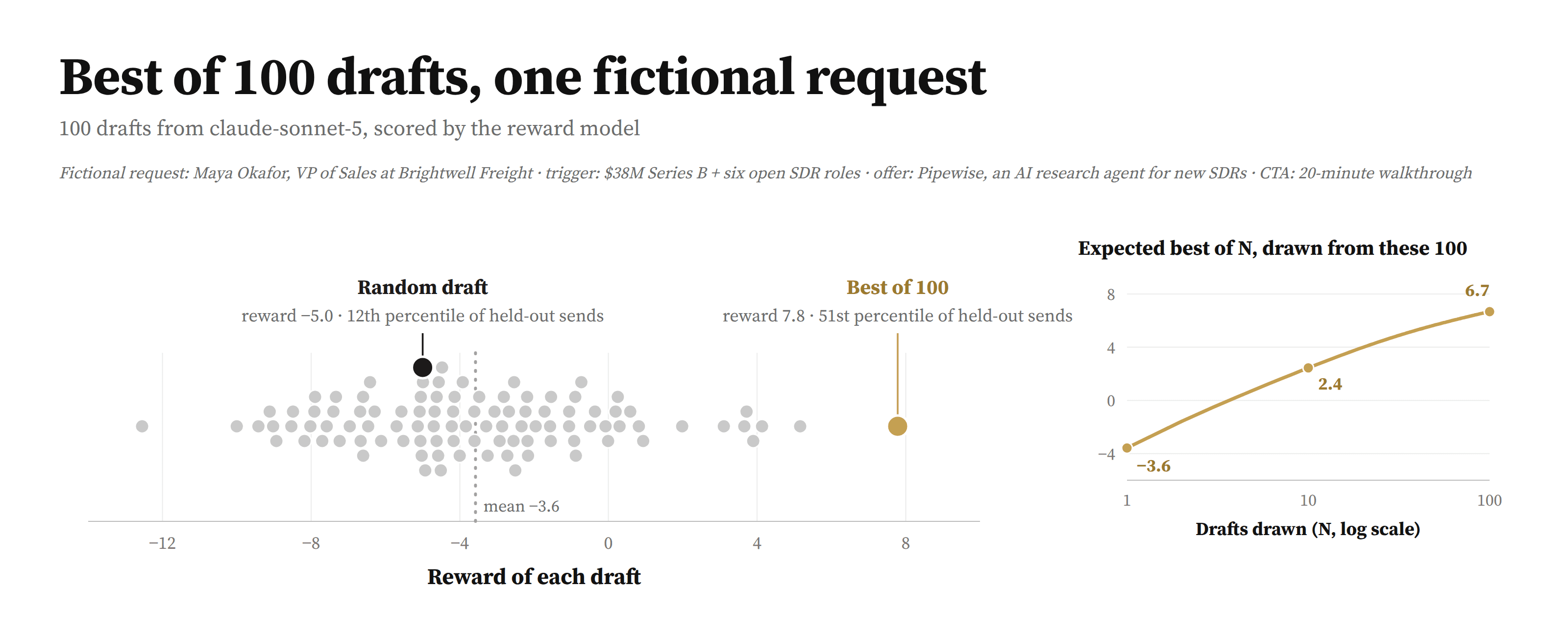
Figure 9: Left: the reward of each of 100 drafts sampled from claude-sonnet-5 (temperature 1.0) for the fictional request in Figure 1, with the random draft and the top-scoring draft marked. Right: the expected reward of the best draft if you drew N drafts at random, with replacement, from these same 100. N = 1 is the average draft (−3.6). The curve is computed exactly from this example's scores, not smoothed: ten drafts already get most of the gain (2.4), and a hundred reach 6.7 on average, below the 7.8 maximum because a random set of 100 often misses the single best draft.

Projected through the reply-rate fit in Figure 4, the random draft would get a reply about 0.7% of the time and the best of 100 about 1.5%, more than twice as often. That is a projection, not a measured lift, but it shows what an instant, trustworthy score unlocks. In the rest of this series, we'll share how we put this reward to work in the agent beyond best-of-N.